Tutorial
define a dimarray
A ``DimArray`` can be defined just like a numpy array, with additional information about its axes, which can be given via axes and dims parameters.
>>> from dimarray import DimArray, Dataset
>>> a = DimArray([[1.,2,3], [4,5,6]], axes=[['a', 'b'], [1950, 1960, 1970]], dims=['variable', 'time'])
>>> a
dimarray: 6 non-null elements (0 null)
0 / variable (2): 'a' to 'b'
1 / time (3): 1950 to 1970
array([[1., 2., 3.],
       [4., 5., 6.]])
data structure
Array data are stored in a values attribute:
>>> a.values
array([[1., 2., 3.],
       [4., 5., 6.]])
while its axes are stored in axes
>>> a.axes
0 / variable (2): 'a' to 'b'
1 / time (3): 1950 to 1970
As a convenience, axis labels can be accessed directly by name, as an alias for a.axes[‘time’].values:
>>> a.time
array([1950, 1960, 1970])
For more information refer to section on DimArray class (as well as dimarray.Axis and dimarray.Axes)
numpy-like attributes
Numpy-like attributes dtype, shape, size or ndim are defined, and are now augmented with dims and labels
>>> a.shape
(2, 3)
>>> a.dims      # grab axis names (the dimensions)
('variable', 'time')
>>> a.labels   # grab axis values
(array(['a', 'b'], dtype=object), array([1950, 1960, 1970]))
indexing
Indexing works on labels just as expected, including slice and boolean array.
>>> a['b', 1970]
6.0
but integer-index is always possible via ix toogle between labels- and position-based indexing:
>>> a.ix[0, -1]
3.0
See also
transformation
Standard numpy transformations are defined, and now accept axis name:
>>> a.mean(axis='time')
dimarray: 2 non-null elements (0 null)
0 / variable (2): 'a' to 'b'
array([2., 5.])
and can ignore missing values (nans) if asked to:
>>> import numpy as np
>>> a['a',1950] = np.nan
>>> a.mean(axis='time', skipna=True)
dimarray: 2 non-null elements (0 null)
0 / variable (2): 'a' to 'b'
array([2.5, 5. ])
See also
alignment in operations
During an operation, arrays are automatically re-indexed to span the same axis domain, with nan filling if needed. This is quite useful when working with partly-overlapping time series or with incomplete sets of items.
>>> yearly_data = DimArray([0, 1, 2], axes=[[1950, 1960, 1970]], dims=['year'])
>>> incomplete_yearly_data = DimArray([10, 100], axes=[[1950, 1960]], dims=['year']) # last year 1970 is missing
>>> yearly_data + incomplete_yearly_data
dimarray: 2 non-null elements (1 null)
0 / year (3): 1950 to 1970
array([ 10., 101.,  nan])
See also
A check is also performed on the dimensions, to ensure consistency of the data. If dimensions do not match this is not interpreted as an error but rather as a combination of dimensions. For example, you may want to combine some fixed spatial pattern (such as an EOF) with a time-varying time series (the principal component). Or you may want to combine results from a sensitivity analysis where several parameters have been varied (one dimension per parameter). Here a minimal example where the above-define annual variable is combined with seasonally-varying data (camping summer and winter prices).
Arrays are said to be broadcast:
>>> seasonal_data = DimArray([10, 100], axes=[['winter','summer']], dims=['season'])
>>> combined_data = yearly_data * seasonal_data
>>> combined_data
dimarray: 6 non-null elements (0 null)
0 / year (3): 1950 to 1970
1 / season (2): 'winter' to 'summer'
array([[  0,   0],
       [ 10, 100],
       [ 20, 200]])
See also
dataset
Changed in version 0.1.9.
As a commodity, the `Dataset` class is an ordered dictionary of DimArray instances which all share a common set of axes.
>>> dataset = Dataset({'combined_data':combined_data, 'yearly_data':yearly_data,'seasonal_data':seasonal_data})
>>> dataset
Dataset of 3 variables
0 / season (2): 'winter' to 'summer'
1 / year (3): 1950 to 1970
seasonal_data: ('season',)
combined_data: ('year', 'season')
yearly_data: ('year',)
At initialization, the arrays are aligned on-the-fly. Later on, it is up to the user to reindex the arrays to match the Dataset axes.
Note
since Dataset elements share the same axes, any axis modification will also impact all contained DimArray instances. If this behaviour is not desired, a copy should be made.
netCDF reading and writing
A natural I/O format for such an array is netCDF, common in geophysics, which rely on the netCDF4 package. If netCDF4 is installed (much recommanded), a dataset can easily read and write to the netCDF format:
>>> dataset.write_nc('/tmp/test.nc', mode='w')
>>> import dimarray as da
>>> da.read_nc('/tmp/test.nc', 'combined_data')
dimarray: 6 non-null elements (0 null)
0 / year (3): 1950 to 1970
1 / season (2): u'winter' to u'summer'
array([[  0,   0],
       [ 10, 100],
       [ 20, 200]])
See also
metadata
It is possible to define and access metadata via the standard . syntax to access an object attribute:
>>> a = DimArray([1, 2])
>>> a.name = 'myarray'
>>> a.units = 'meters'
Any non-private attribute is automatically added to a.attrs ordered dictionary:
>>> a.attrs
OrderedDict([('name', 'myarray'), ('units', 'meters')])
Metadata can also be defined for dimarray.Dataset and dimarray.Axis instances, and will be written to / read from netCDF files.
Note
Metadata that start with an underscore _ or use any protected class attribute as name (e.g. values, axes, dims and so on) must be set directly in attrs.
See also
Metadata for more information.
join arrays
DimArrays can be joined along an existing dimension, we say concatenate (dimarray.concatenate()):
>>> a = DimArray([11, 12, 13], axes=[[1950, 1951, 1952]], dims=['time'])
>>> b = DimArray([14, 15, 16], axes=[[1953, 1954, 1955]], dims=['time'])
>>> da.concatenate((a, b), axis='time')
dimarray: 6 non-null elements (0 null)
0 / time (6): 1950 to 1955
array([11, 12, 13, 14, 15, 16])
or they can be stacked along each other, thereby creating a new dimension (dimarray.stack())
>>> a = DimArray([11, 12, 13], axes=[[1950, 1951, 1952]], dims=['time'])
>>> b = DimArray([21, 22, 23], axes=[[1950, 1951, 1952]], dims=['time'])
>>> da.stack((a, b), axis='items', keys=['a','b'])
dimarray: 6 non-null elements (0 null)
0 / items (2): 'a' to 'b'
1 / time (3): 1950 to 1952
array([[11, 12, 13],
       [21, 22, 23]])
In the above note that new axis values were provided via the parameter keys=. If the common “time” dimension was not fully overlapping, array can be aligned prior to stacking via the align=True parameter.
>>> a = DimArray([11, 12, 13], axes=[[1950, 1951, 1952]], dims=['time'])
>>> b = DimArray([21, 23], axes=[[1950, 1952]], dims=['time'])
>>> c = da.stack((a, b), axis='items', keys=['a','b'], align=True)
>>> c
dimarray: 5 non-null elements (1 null)
0 / items (2): 'a' to 'b'
1 / time (3): 1950 to 1952
array([[11., 12., 13.],
       [21., nan, 23.]])
See also
drop missing data
Say you have data with NaNs:
>>> a = DimArray([[11, np.nan, np.nan],[21,np.nan,23]], axes=[['a','b'],[1950, 1951, 1952]], dims=['items','time'])
>>> a
dimarray: 3 non-null elements (3 null)
0 / items (2): 'a' to 'b'
1 / time (3): 1950 to 1952
array([[11., nan, nan],
       [21., nan, 23.]])
You can drop every column that contains a NaN
>>> a.dropna(axis=1) # drop along columns
dimarray: 2 non-null elements (0 null)
0 / items (2): 'a' to 'b'
1 / time (1): 1950 to 1950
array([[11.],
       [21.]])
or actually control decide to retain only these columns with a minimum number of valid data, here one:
>>> a.dropna(axis=1, minvalid=1) # drop every column with less than one valid data
dimarray: 3 non-null elements (1 null)
0 / items (2): 'a' to 'b'
1 / time (2): 1950 to 1952
array([[11., nan],
       [21., 23.]])
See also
reshaping arrays
Additional novelty includes methods to reshaping an array in easy ways, very useful for high-dimensional data analysis.
>>> large_array = DimArray(np.arange(2*2*5*2).reshape(2,2,5,2), dims=('A','B','C','D'))
>>> small_array = large_array.reshape('A,D','B,C')
>>> small_array
dimarray: 40 non-null elements (0 null)
0 / A,D (4): (0, 0) to (1, 1)
1 / B,C (10): (0, 0) to (1, 4)
array([[ 0,  2,  4,  6,  8, 10, 12, 14, 16, 18],
       [ 1,  3,  5,  7,  9, 11, 13, 15, 17, 19],
       [20, 22, 24, 26, 28, 30, 32, 34, 36, 38],
       [21, 23, 25, 27, 29, 31, 33, 35, 37, 39]])
See also
interfacing with pandas
For things that pandas does better, such as pretty printing, I/O to many formats, and 2-D data analysis, just use the dimarray.DimArray.to_pandas() method. In the ipython notebook it also has a nice html rendering.
>>> small_array.to_pandas()
B     0                   1
C     0   1   2   3   4   0   1   2   3   4
A D
0 0   0   2   4   6   8  10  12  14  16  18
  1   1   3   5   7   9  11  13  15  17  19
1 0  20  22  24  26  28  30  32  34  36  38
  1  21  23  25  27  29  31  33  35  37  39
| B | 0 | 1 | |||||||||
|---|---|---|---|---|---|---|---|---|---|---|---|
| C | 0 | 1 | 2 | 3 | 4 | 0 | 1 | 2 | 3 | 4 | |
| A | D | ||||||||||
| 0 | 0 | 0 | 2 | 4 | 6 | 8 | 10 | 12 | 14 | 16 | 18 |
| 1 | 1 | 3 | 5 | 7 | 9 | 11 | 13 | 15 | 17 | 19 | |
| 1 | 0 | 20 | 22 | 24 | 26 | 28 | 30 | 32 | 34 | 36 | 38 |
| 1 | 21 | 23 | 25 | 27 | 29 | 31 | 33 | 35 | 37 | 39 | |
And dimarray.DimArray.from_pandas() works to convert pandas objects to DimArray (also supports MultiIndex):
>>> import pandas as pd
>>> s = pd.DataFrame([[1,2],[3,4]], index=['a','b'], columns=[1950, 1960])
>>> da.from_pandas(s)
dimarray: 4 non-null elements (0 null)
0 / x0 (2): 'a' to 'b'
1 / x1 (2): 1950 to 1960
array([[1, 2],
       [3, 4]])
plotting
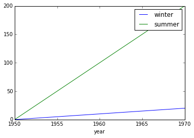
dimarray comes with basic plotting facility. For 1-D and 2-D data, it simplies interfaces pandas’ plot command (therefore pandas needs to be installed to use it). From the example above:
>>> %pylab # doctest: +SKIP
>>> %matplotlib inline # doctest: +SKIP
>>> a = dataset['combined_data']
>>> a.plot() # doctest: +SKIP
Using matplotlib backend: TkAgg
Populating the interactive namespace from numpy and matplotlib
[<matplotlib.lines.Line2D at 0x7f729cffdd50>,
 <matplotlib.lines.Line2D at 0x7f729cffded0>]
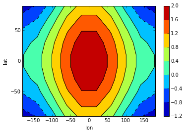
In addition, it can also display 2-D data via its methods contour, contourf and pcolor mapped from matplotlib.
>>> # create some data
>>> lon = np.linspace(-180, 180, 10)
>>> lat = np.linspace(-90, 90, 10)
>>> LON, LAT = np.meshgrid(lon, lat)
>>> DATA = np.cos(np.radians(LON)) + np.cos(np.radians(LAT))
>>> # define dimarray
>>> a = DimArray(DATA, axes=[lat, lon], dims=['lat','lon'])
>>> # plot the data
>>> c = a.contourf()
>>> colorbar(c)  # explicit colorbar creation  # doctest: +SKIP
>>> a.contour(colors='k') # doctest: +SKIP
/home/perrette/glacierenv/local/lib/python2.7/site-packages/matplotlib/collections.py:650: FutureWarning: elementwise comparison failed; returning scalar instead, but in the future will perform elementwise comparison
  if self._edgecolors_original != str('face'):
<matplotlib.contour.QuadContourSet instance at 0x7f729ce46b00>/home/perrette/glacierenv/local/lib/python2.7/site-packages/matplotlib/collections.py:590: FutureWarning: elementwise comparison failed; returning scalar instead, but in the future will perform elementwise comparison
  if self._edgecolors == str('face'):
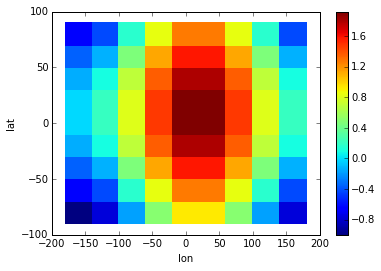
>>> # plot the data
>>> a.pcolor(colorbar=True)  # colorbar as keyword argument # doctest: +SKIP
<matplotlib.collections.QuadMesh at 0x7f729cd3aa10>
For more information, you can use inline help (help() or ?) or refer to Advanced topics and Reference API